Celestial mechanics and coordinate system conventions
Note
We mostly follow the notation and conventions defined in Murray and Correia (2010).
The Kepler ellipse
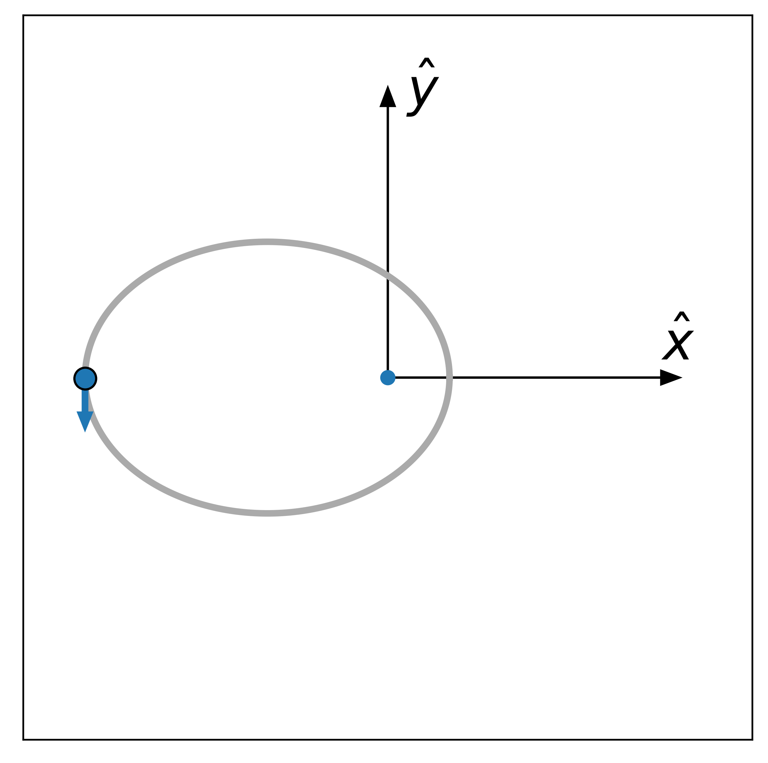
We won’t review the derivation or solution of the Kepler problem – we recommend sections 1–3 in Murray and Correia (2010) – and instead start from the fact that the shape of a single Keplerian orbit is an ellipse. The position of an orbiting body in its orbital plane is given by the vector \(\boldsymbol{r} = \left(x, y, 0\right)\). The basis for this coordinate system is defined such that \(\hat{x}\) lies along the major axis of the orbit ellipse, increasing from apocenter to pericenter. The basis vector \(\hat{z}\) is aligned with the orbital angular momentum and is perpendicular to \(\hat{x}\), and \(\hat{y}\) lies in the orbital plane and is perpendicular to both \(\hat{x}\) and \(\hat{z}\). Orbital motion is therefore constrained to the \(x\)-\(y\) plane by construction. See figure below: the grey ellipse represents the orbit of the (blue) body, with the arrow indicating the direction of the orbit. The \(x\)-\(y\) basis is shown as dark black arrows relative to the reference point (typically the center of mass):
(Source code, png)
The position of the body on its orbit, \(\boldsymbol{r} = (x, y, 0)\), can be expressed in terms of its orbital elements and time. First, we’ll define the angles typically used in expressing solutions to the Kepler problem. These are the mean anomaly, \(M\), the eccentric anomaly, \(E\), and the true anomaly, \(f\). These can be expressed in terms of the period of the orbit \(P\), a time \(t\), a reference epoch \(t_0\), the orbital eccentricity \(e\), and the semi-major axis \(a\):
In the above, \(r\) is the distance of the body from the focus of the ellipse closest to pericenter. \(M_0\) is the mean anomaly or phase of the orbit at the reference epoch. Using the above definitions, the position and velocity of the body in the orbital plane coordinates is given by:
Observer or reference plane coordinates
Of course, orbits of celestial bodies are generically rotated in with respect to the observer’s perspective (usually assumed to be sitting at the solar system barycenter). The orientation of the orbit is therefore defined in terms of orbital elements that rotate between the orbital plane \((x, y, z)\) system and another reference coordinate system \((X, Y, Z)\). In the new \((X, Y, Z)\), the reference plane must be defined. We use the tangent plane at a point on the celestial sphere as the reference plane, with the observer sitting along the positive \(Z\) axis (see Figure 7 in Murray and Correia (2010)). At a given tangent point, the \(\hat{X}\) direction is aligned with North, and \(\hat{Y}\) with the East direction of the celestial coordinates used.
The angles that define the rotation from \((x, y, z)\) to \((X, Y, Z)\) are the angular components of the orbital elements: longitude of the ascending node, \(\Omega\), the argument of pericenter, \(\omega\), and the inclination, \(i\). The full transformation is then a series of three rotations: (1) rotate by \(\omega\) around the \(z\) axis to align \(x'\) with the line of nodes, (2) rotate by \(i\) around \(x'\) to make the \(x'', y''\) plane coincident with the reference plane, and (3) rotate by \(\Omega\) around \(z''\) to align \(x'''\) with \(X\). So, to transform an orbit from its orbital plane to the reference system, the full transformation is given by the composition of three rotation matrices:
where
See also: