Getting started with twobody

For the examples below, we’ll need the following imports:

>>> import astropy.units as u
>>> from astropy.time import Time
>>> import astropy.coordinates as coord
>>> import matplotlib.pyplot as plt
>>> import numpy as np

Compute and plot a radial velocity curve given orbital elements

We work with Keplerian orbits using the KeplerOrbit class, which accepts orbital elements on creation:

>>> from twobody import KeplerOrbit
>>> orb = KeplerOrbit(P=1.5*u.year, e=0.67,
...                   omega=17.14*u.deg, i=65*u.deg, Omega=0*u.deg,
...                   M0=35.824*u.deg, t0=Time('J2015.0'))

The elements are described in more detail in Celestial mechanics and coordinate system conventions, but, briefly, P is the orbital period, e is the eccentricity, omega is the argument of pericenter, i is the inclination of the orbital plane, Omega is the longitude of the ascending node (which has no effect on the radial velocity curve, so we set to 0), M0 is the phase of the orbit at the reference time t0. All of the specific values of the above parameters were made up at random. Note that we haven’t specified a semi-major axis, so the absolute scale of the radial velocity variations isn’t specified. 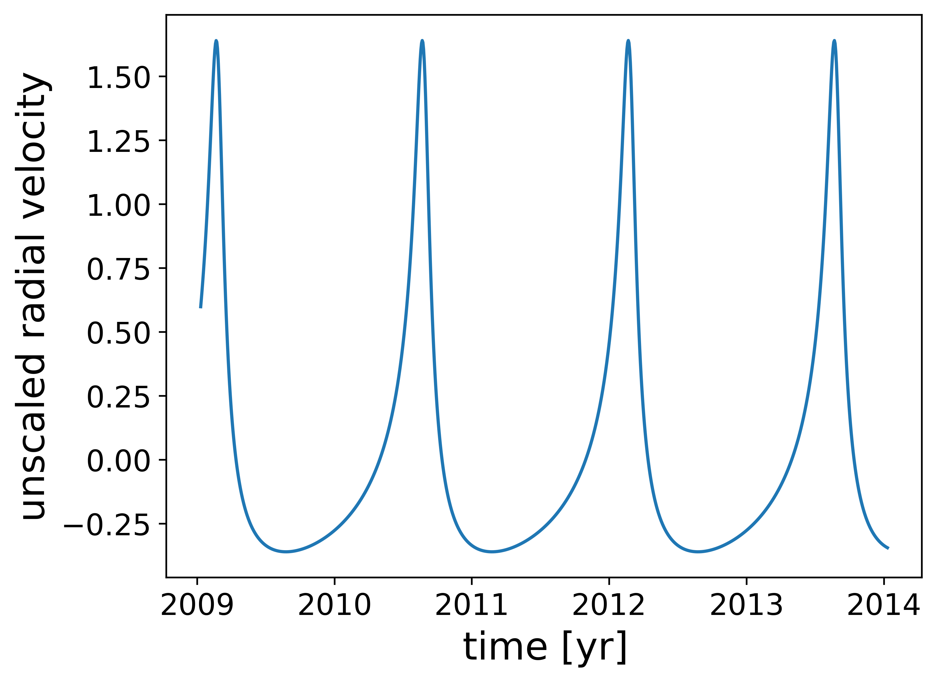This is useful if you are fitting for the velocity semi-amplitude K and systemic velocity of the barycenter v0, which are just linear parameters in the unscaled radial velocity. We can compute the unscaled radial velocity by specifying an array of times to the unscaled_radial_velocity method:

>>> t = Time('2009-01-10') + np.linspace(0, 5, 1024) * u.year
>>> unscaled_rv = orb.unscaled_radial_velocity(t)

Let’s plot these values to visualize:

>>> fig,ax = plt.subplots(1, 1) 
>>> ax.plot(t.datetime, unscaled_rv.value, marker='') 
>>> ax.set_xlabel('time [{0:latex_inline}]'.format(u.year)) 
>>> ax.set_ylabel('unscaled radial velocity') 

(Source code, png)

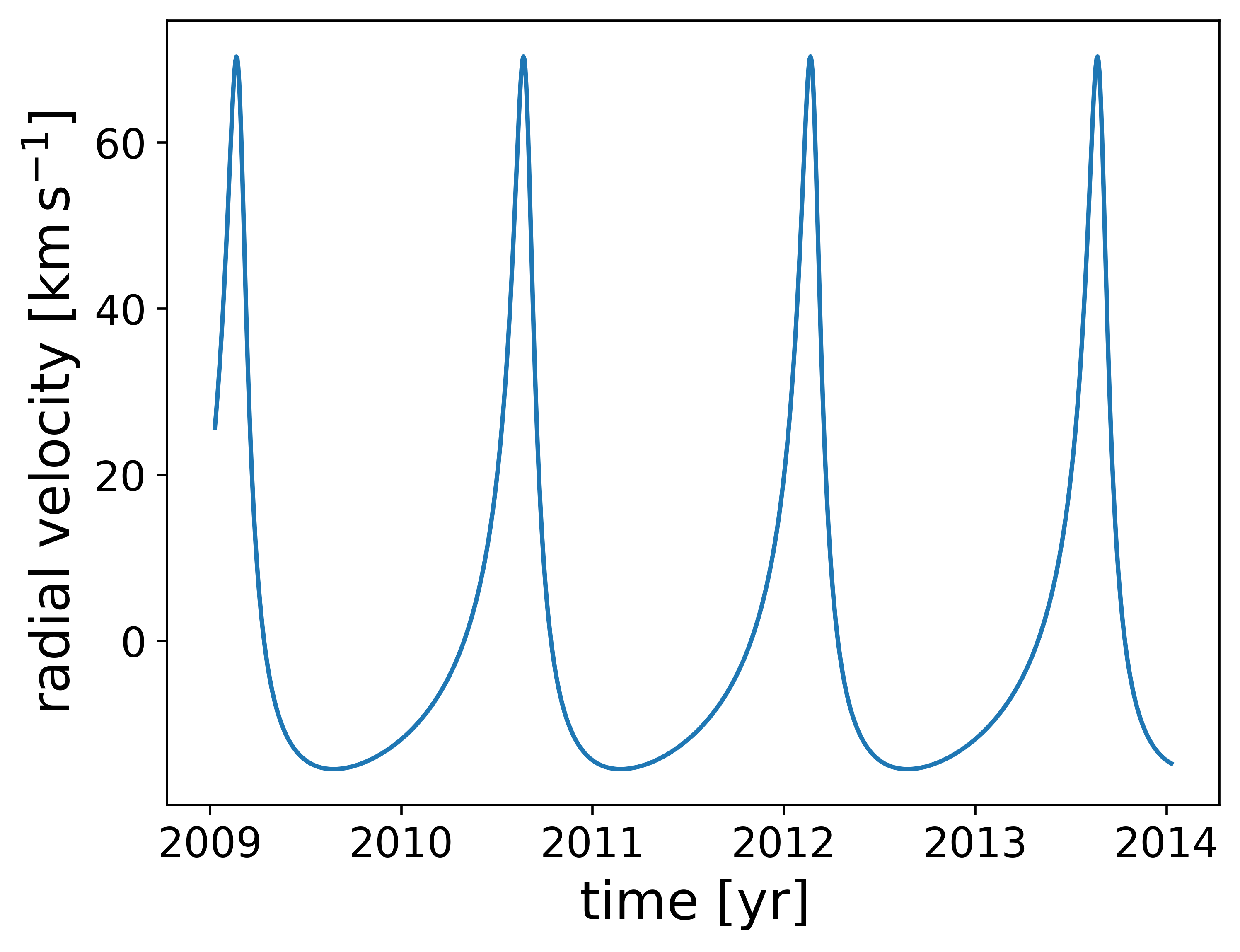
If we do specify the semi-major axis, the velocity amplitude is known and we can compute the actual (scaled) radial velocity curve with the radial_velocity method:

>>> orb = KeplerOrbit(P=1.5*u.year, e=0.67, a=1.77*u.au,
...                   omega=17.14*u.deg, i=65*u.deg, Omega=0*u.deg,
...                   M0=35.824*u.deg, t0=Time('J2015.0'))
>>> fig,ax = plt.subplots(1, 1) 
>>> ax.plot(t.datetime, rv.to(u.km/u.s).value, marker='') 
>>> ax.set_xlabel('time [{0:latex_inline}]'.format(u.year)) 
>>> ax.set_ylabel('radial velocity [{0:latex_inline}]'.format(u.km/u.s)) 

(Source code, png)

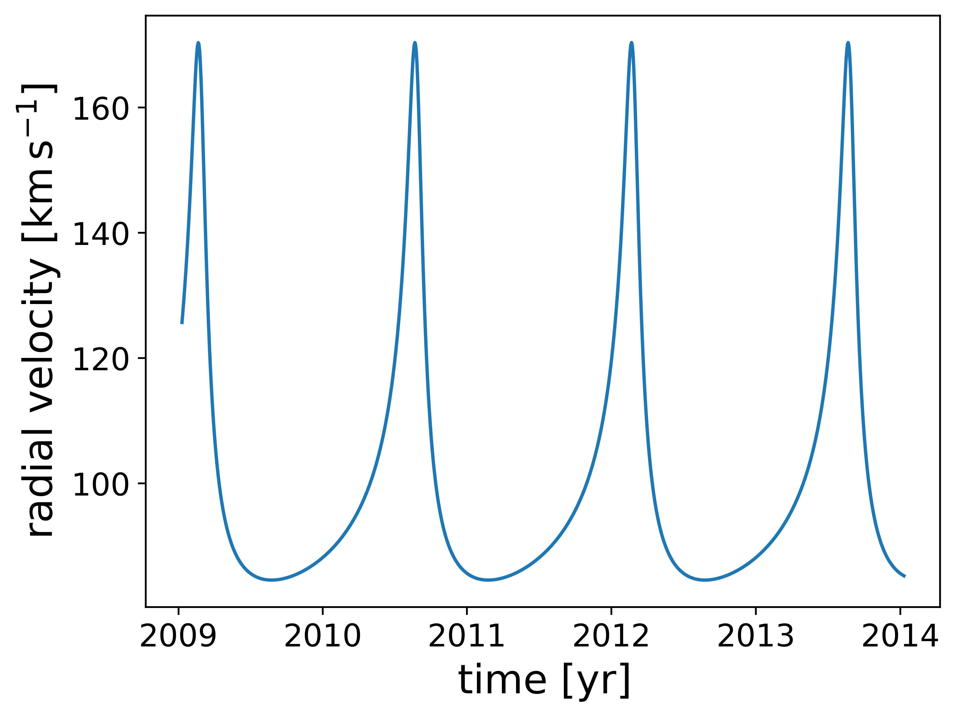
The radial velocities computed above are relative to the barycenter or reference point of the orbit. We can add the barycentric or systemic velocity of the system to the output radial velocities to get the actual line of sight velocities. For example, if the systemic velocity is 100 km/s:

>>> v0 = 100 * u.km/u.s
>>> fig,ax = plt.subplots(1, 1) 
>>> ax.plot(t.datetime, (rv + v0).to(u.km/u.s).value, marker='') 
>>> ax.set_xlabel('time [{0:latex_inline}]'.format(u.year)) 
>>> ax.set_ylabel('radial velocity [{0:latex_inline}]'.format(u.km/u.s)) 

(Source code, png)

Note that both radial_velocity and unscaled_radial_velocity assume that the barycenter does not move tangentially when computing the velocity. That is, the radial velocity computed is actually just \(\dot{Z}\) computed in reference plane coordinates (see Celestial mechanics and coordinate system conventions). For sources that move appreciable over the baseline of observations, the observed line-of-sight velocity will change slightly because of spherical projection effects, but the differences will be small. See the docstring of radial_velocity for more information.

Compute and plot an astrometric orbit curve given orbital elements and barycenter motion

We again start by creating a KeplerOrbit instance (see example above) to represent a Keplerian orbit. However, to compute an astrometric orbit, we also need to specify the location and velocity of the system barycenter at some reference epoch. This epoch can be different from the epoch from which the orbital elements are defined. To specify the barycenter, we therefore need to create an astropy.coordinates object, and an astropy.time.Time object. Here, let’s assume our barycenter reference epoch is Jan. 1, 2014, and make up some coordinates and velocity components for the barycenter:

>>> from twobody import Barycenter
>>> origin = coord.ICRS(ra=14.745*u.deg, dec=71.512*u.deg,
...                     distance=71.634*u.pc,
...                     pm_ra_cosdec=32.123*u.mas/u.yr,
...                     pm_dec=86.63*u.mas/u.yr,
...                     radial_velocity=17.4123*u.km/u.s)
>>> barycen = Barycenter(origin=origin, t0=Time('J2014'))

We can pass this in when creating a KeplerOrbit object so that the orbit object knows about the motion of the barycenter:

>>> from twobody import KeplerOrbit
>>> orb = KeplerOrbit(P=1.5*u.year, a=1.83*u.au, e=0.67,
...                   omega=17.14*u.deg, i=65*u.deg, Omega=0*u.deg,
...                   M0=35.824*u.deg, t0=Time('J2015.0'),
...                   barycenter=barycen)

We can then compute the position and velocity of the orbiting body at specified times in the ICRS frame using the icrs method:

>>> t = Time('J2010') + np.linspace(0, 8*orb.P.value, 10000)*orb.P.unit
>>> orb_icrs = orb.icrs(t)

This gives us the ICRS position and velocity components of the source, but sometimes we might instead want to work in an “offset” frame centered on the reference location of the barycenter, i.e. a spherical coordinate system aligned with the ICRS, but with (0,0) at the location of the barycenter at the specified epoch (J2014). We can transform to this frame using the astropy.coordinates.SkyOffsetFrame (this requires Astropy version 3.0 or higher):

>>> offset_frame = coord.SkyOffsetFrame(origin=origin)
>>> orb_offset = orb_icrs.transform_to(offset_frame)

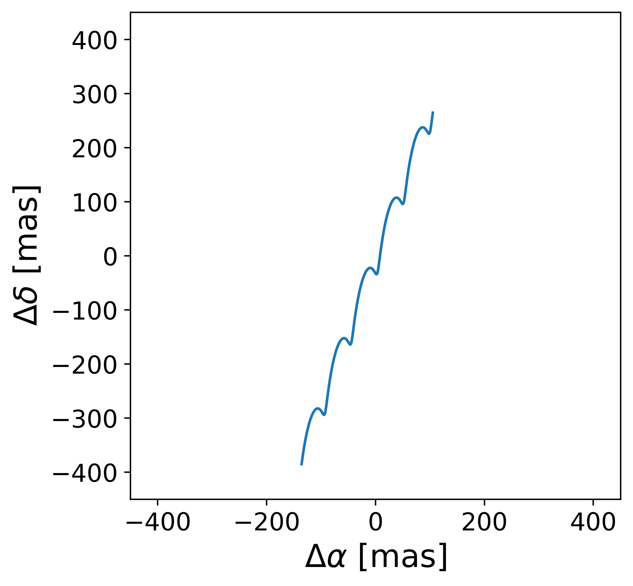
We can then plot the astrometric orbit, including barycenter motion, in the offset ICRS frame:

>>> fig,ax = plt.subplots(1, 1) 
>>> ax.plot(offset_frame.lon.wrap_at(180*u.deg).milliarcsecond,
...         offset_frame.lat.milliarcsecond, marker='') 
>>> ax.set_xlabel(r'$\Delta\alpha$ [{0:latex_inline}]'.format(u.mas)) 
>>> ax.set_ylabel(r'$\Delta\delta$ [{0:latex_inline}]'.format(u.mas)) 
>>> ax.set_xlim(-450, 450) 
>>> ax.set_ylim(-450, 450) 

(Source code, png)